 Data Wrangler
Teapot Dome against the clock
The same Teapot Dome delivery the Outrider had already loaded once, in 14.7 minutes. A day spent making it faster, run after run, measured every time. At the end of it the first table was in at 0.7 minutes instead of 3.9, and every row of the delivery by 8.0 minutes. Not all of that is speed. Some of it is a smaller herd, and this page says which is which.
Faster is a trail. You find out where it goes by riding it.
The question that started it
Watching the Teapot load, the trail boss asked why every plan was worked out before any of them was carried out. The answer was that code checked all 27 saved loading plans, one after another, reading every file in full, before a single row went in: 203 seconds of nothing loading. Then the agent and the loader took turns, never working at the same time.
So the loader got its own lane. Code now lists what it will load in seconds (16 on the final run), the loader starts on the well headers at once, and the remaining plans are checked while the first ones load. Each one loads the moment its own check passes. The first table went from minute 3.9 to minute 0.7.
Where the minutes went
What made the difference
-
Load while you plan
The loader runs on its own every few seconds, whatever the agent is doing, and code's saved plans are checked in the background. First table at 0.7 minutes, not 3.9. the trail boss's question
-
Documents side by side, each on its own
Every document folder used to be read one after the other, inside the same program as everything else. Now each folder gets its own process, and they run side by side. The 318 well reports started at minute 0.8 instead of 11.6. Timed on its own, in a process of its own, the 1,202-file well-log folder took 100 seconds.
-
No table waits for a slower one
Tables loaded in batches, and each batch waited for its slowest member. 42,176 survey stations spent four minutes loading while small tables queued behind them. Now a table starts the moment a slot is free.
-
Stop doing work twice
The production volumes load went from 86 seconds to 59. An 11.6-second re-read of the 210,507-row production workbook, done only to learn its column names, is gone. So is repairing 876,480 cells that had nothing to repair: that step fell from 24 seconds to 6.
-
Folders stop waiting on each other
A folder's rows would not load while another folder's rows still sat unchecked, so the well reports waited for the well logs. Under the session rule, which checks each folder itself as soon as it is read, a delivery's own folders no longer hold each other up.
Throwing the rope and missing
Not every throw caught anything. The afternoon had runs slower than the original, and it is fairer to say so than to leave them out.
-
More at once made it slower
Three document folders, four table loads and four plan checks at once, all writing to one database. The database is SQL Server Express, which uses at most four cores however many the machine has. A 16-row load that takes 0.9 seconds on its own took 48 seconds in that crowd. The fix was to do less at once: two folders, three tables.
-
A runner that never came back
One document runner hit a Windows access error while starting its helper processes, then waited on them for thirteen minutes. The Python it ran on was the Microsoft Store edition, which starts every process through its own launcher, so Python was reinstalled from python.org. And a runner that goes silent for five minutes is now stopped and tried once more.
-
137 map layers, 848 features, eleven minutes
The geodatabase held 137 map layers. Loading them took eleven minutes, most of it one database statement per feature. The trail boss's answer was that only a few layers were wanted anyway, so the final run left the geodatabase out. “let me select what layers to load”
A smaller herd
The final run did less than the original, by the trail boss's choice. Its 8.0 minutes and the original's 14.7 are not the same job, so here is the difference.
| Table | Original | Final run | Why |
|---|---|---|---|
| Trimmed on purpose | |||
| dv_seis_horizon_grid | 241,587 | 0 | 3D horizons, left out: “we actually don't need it” |
| dv_seis_horizon | 9 | 0 | the same horizons |
| dv_well_core_photo | 208 | 40 | cut down to the core slab photographs, all 40 of them loaded: “We are only interested in the slabs” |
| Short, and not on purpose | |||
| dv_seis_set / dv_seis_line | 2 / 6 | 1 / 1 | under investigation; see below |
| Everything else — the same row for row | |||
| dv_well | 1,351 | 1,351 | well headers |
| dv_prod_volume | 108,177 | 108,177 | last 36 producing months per well |
| dv_prod_entity | 1,264 | 1,264 | production entities |
| dv_well_dir_srvy_sta | 40,092 | 40,092 | directional survey stations |
| dv_well_log_curve | 8,778 | 8,778 | log curves |
| dv_well_formation_top | 7,405 | 7,405 | formation tops |
| dv_well_dip | 1,945 | 1,945 | FMI dip picks, from the nine dip spreadsheets |
| dv_reservoir | 9 | 9 | reservoirs, from ReservoirData 2005 |
| dv_reservoir_property | 193 | 193 | their properties |
| dv_strat_column | 30 | 30 | the Teapot geologic column |
| dv_well_log | 1,174 | 1,174 | logs |
| and the same counts for survey headers, cores and core samples, checkshots, casing and drill-stem tests | |||
What can be compared like for like is the timeline above: the first table at 0.7 minutes instead of 3.9; the well reports starting at 0.8 instead of 11.6; and 203 seconds of plan-checking before anything loaded, gone.
What three of those tables hold
Row counts say little about what a geologist gets. These three come from Teapot Dome spreadsheets that fit no ordinary loader, and the original load built a table for each.
The geologic column
Thirty units from the Steele Shale at the surface to the Granite at 7,085 feet, each with its top, its thickness, its period, and whether it produces. Shannon, the 2nd Wall Creek and the Tensleep are the current producers. The Tensleep, the deepest of them, has its top at 5,525 feet and is 320 feet thick. Each unit links to its reservoir row where there is one.
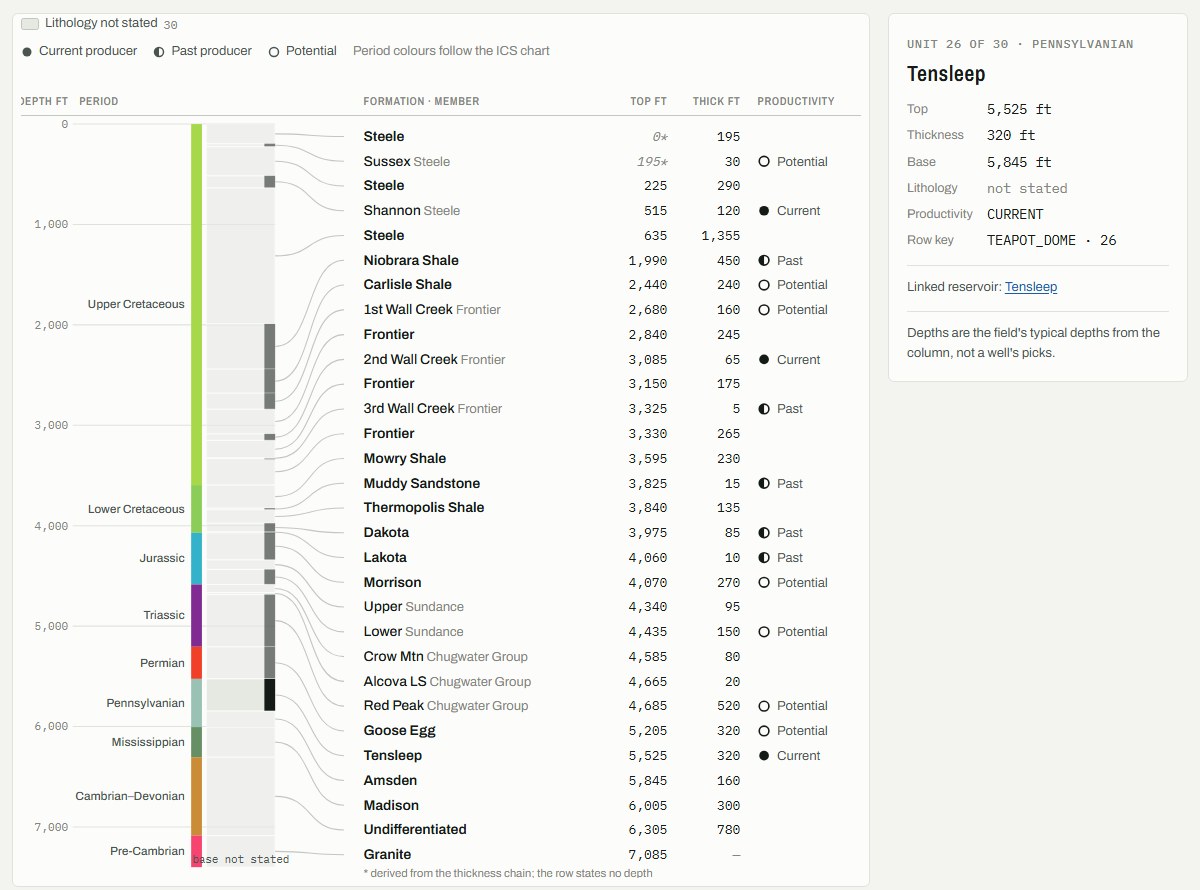
dv_strat_column, 30 rows. The wide lithology band is empty here: the rock
types are read from the workbook's cell colours by a separate step that was not run
on this load.
The reservoirs
Nine reservoirs, with 193 properties between them, as of 2005: oil originally in place, how much has been produced, porosity, permeability, pressure, depth and well counts. Where the sheet says “N/A – Fractured” instead of a porosity, that is what the table says too; it is never turned into a number. The Tensleep alone carries 22 properties: 3.83 million barrels in place, 1.84 million produced (48%), 8% porosity, 80 millidarcies, 2,350 psi, 190°F, 32° API oil and 13 producing wells.
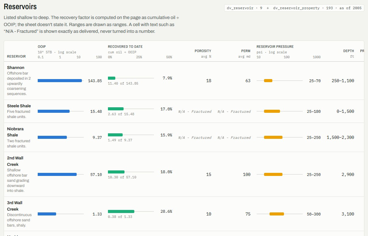
dv_reservoir, 9 rows. The share recovered is worked out on the
page from cumulative oil and oil in place; the sheet does not state it.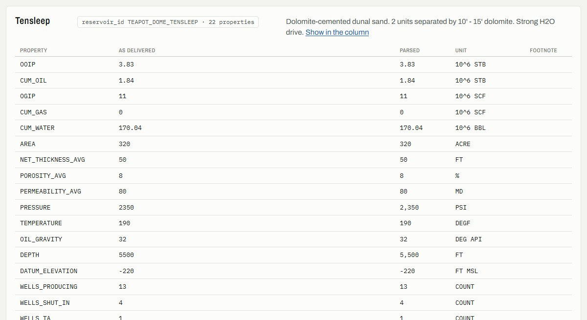
dv_reservoir_property: each value as delivered, as parsed, and in
its unit. Text answers such as a depletion strategy stay text.The FMI dips
Nine spreadsheets of picks from an FMI image log in one well, 48-X-28: 1,945 dips, each a depth, a true dip and a direction. 640 sedimentary bedding, 547 inter-dune bedding, 88 bed boundaries, 95 natural fractures, 38 drilling-induced fractures, and 537 the workbook calls “BorDip” without saying what it means, kept under that name. Drawn as a tadpole plot against the well's formation tops, with rose diagrams of dip direction. Over the Tensleep, the natural fractures strike 099°/279°, and the drilling-induced fractures strike 103°/283°, the direction of maximum horizontal stress.
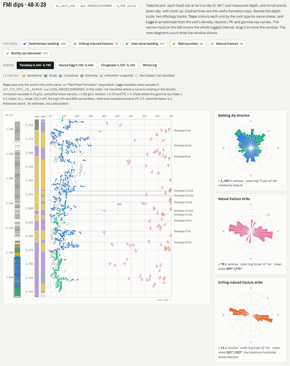
dv_well_dip, 1,945 rows, all for well 49025231950000. Beside the
depth scale: rock type from the formation names, and an estimate from the well's
density, neutron and gamma-ray logs.The ceiling
By the end of the day the loading itself was held up by one thing: the database. With the work spread out, table loads, document reads and document loads all queue for the same four cores. More parallel work past that point makes a run slower, not faster, and the afternoon measured exactly that.
The trail boss put it plainly: “IF we are constrained by the database we can't do much better.” The next step up is a database edition that isn't capped at four cores, and that is the trail boss's call.
Still on the trail
The seismic lines
The original loaded 2 seismic surveys and 6 lines; the final run loaded 1 and 1. It happened on two runs in a row, once without any database collision, so it is a real fault and not bad luck.
2.7 minutes of paperwork
Every row was in at 8.0 minutes; the session ended at 10.7. The difference is the agent's paperwork on the rest of the FMI folder. The FMI dip picks themselves loaded, all 1,945 of them, into the dip table the original load built for them. Left over were the log print files, a presentation, an image, and five fracture spreadsheets, which the original run set aside as well. Code will not let the agent finish until every file is loaded or set aside with a reason, and its set-asides kept overlapping and missing a few, on both runs. Tonight that took 25 turns and 51 cents, part of why the run cost $1.33 against $0.52 on the best run of the day. The five fracture spreadsheets deserve a real look: set aside twice is not the same as not loadable.
Which of two duplicate readings wins
The production row counts match the original exactly, but on a few duplicate well-month readings in the source sheet a different value was kept: oil 11 barrels higher, water 389 barrels lower, over the whole delivery. Whichever row loads first wins, and the load order changed. That should be a rule, not a matter of timing.
Check the tally yourself
Every number on this page comes from the two databases after their runs, from the start and finish times the database recorded for each item, or from a profile of a single load run on its own. The original is the run of 17 September; the final run is the last of 18 September, with the same saved plans, the same standing instructions and the trail boss's earlier answers applied to its cards.
Every row in by eight minutes, the first one in under one, and a clear view of the fence at the far end.
The Outrider waters the horses. The database has four cores, and it is using all of them.